Solar position#
The position of the sun in the sky as seen by an observed on Earth can be described using two angles:
the solar elevation (γS): angle between the sun and the horizontal plane
the solar azimuth (ψS): angle between the projection of the sun on the horizontal plane and the south direction
The complementary angle of the solar elevation angle is often for convenience in trigonometric calculations, which is the zenith angle: θZ = 90° - γS.

The elevation and azimuth angles depend on the location (latitude and longitude), date, and time of day. However, the Sun’s position in the sky as seen by an observer doesn’t exactly match its true position relative to Earth, as the Sun’s rays are refracted as they pass through Earth’s atmosphere. Atmospheric refraction slightly increases the Sun’s elevation angle. So, we need to distinguish between two types of elevation/zenith angles:
True elevation/zenith angle – based on the actual geometric position of the Sun.
Apparent elevation/zenith angle – sun position accounting for atmospheric refraction.
For more information on atmospheric refraction, the reader is referred to atmospheric refraction.
Solar position algorithms (SPAs) are mathematical models used to accurately calculate the position of the sun at any given time and location on Earth. These algorithms determine the key solar angles such as zenith, elevation, and azimuth. Knowing these angles is crucial for applications in solar energy, climate modeling, architecture, and astronomy. Solar position algorithms account for the Earth’s irregular rotation around the Sun based on historical observations. This has caused users to develop different algorithms with different sets of coefficients that are accurate for different time periods.
In general, SPAs can take as input:
Geographic coordinates (latitude and longitude)
Date and time
Atmospheric conditions (temperature and pressure)
Elevation above sea level
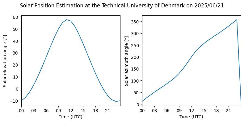
Below, we calculate the solar position at the Technical University of Denmark on 2025/06/21, using the Michalsky algorithm [1].
Show code cell source
import pandas as pd
import matplotlib.pyplot as plt
import solposx
from pvlib.location import Location
import matplotlib.dates as mdates

# Definition of Location object
site = Location(55.79, 12.52, 'UTC', 50, 'DTU, Denmark') # latitude, longitude, time_zone, altitude, name

# Definition of a time range of simulation
times = pd.date_range('2025-06-21 00:00:00', '2025-06-22 00:00:00', freq='h', tz=site.tz)

# Calculate solar position
solpos = solposx.solarposition.michalsky(times, site.latitude, site.longitude)

# Plots for solar zenith and solar azimuth angles
fig, axes = plt.subplots(1, 2, figsize=(8, 4))
fig.suptitle('Solar Position Estimation at the Technical University of Denmark on 2025/06/21')

# plot for solar elevation angle
axes[0].plot(solpos.elevation)
axes[0].set_ylabel('Solar elevation angle [°]')

# plot for solar azimuth angle
axes[1].plot(solpos.azimuth)
axes[1].set_ylabel('Solar azimuth angle [°]')

# format plot
for ax in axes:
    ax.set_xlabel('Time (UTC)')
    ax.xaxis.set_major_formatter(mdates.DateFormatter('%H'))
    ax.set_xlim(pd.Timestamp('2025-06-21 00:00:00'), pd.Timestamp('2025-06-21 23:59:00'))

plt.tight_layout()
plt.show()
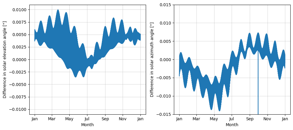
Comparison of two different SPAs#
Compare the accuracy of Skyfield [2] (high-precision tool for calculating the solar position) with the Michalsky algorithm for an entire year. The metric which will be used for the comparison is the root mean square deviation (RMSD).
times = pd.date_range('2025-01-01 00:00:00', '2025-12-31 23:59:00', freq='h', tz='UTC')

michalsky = solposx.solarposition.michalsky(times, site.latitude, site.longitude)
skyfield = solposx.solarposition.skyfield(times, site.latitude, site.longitude)

comparison = solposx.tools.calc_error(michalsky['elevation'], michalsky['azimuth'], skyfield['elevation'], skyfield['azimuth'])
Show code cell output
[ ] 0% de440.bsp
[#### ] 13% de440.bsp
[############ ] 36% de440.bsp
[################## ] 55% de440.bsp
[####################### ] 71% de440.bsp
[############################# ] 88% de440.bsp
[#################################] 100% de440.bsp
Show code cell source
fig, axes = plt.subplots(1, 2, figsize=(10, 4.5), facecolor='w', edgecolor='k')

axes[0].plot(michalsky['elevation']-skyfield['elevation'])
axes[1].plot(michalsky['azimuth']-skyfield['azimuth'])

axes[0].set_ylabel('Difference in solar elevation angle [°]')
axes[0].set_ylim(-0.011, 0.011)

axes[1].set_ylabel('Difference in solar azimuth angle [°]')
axes[1].set_ylim(-0.015, 0.015)

for ax in axes:
    ax.set_xlabel('Month')
    ax.xaxis.set_major_formatter(mdates.DateFormatter('%b'))
    ax.grid(alpha=0.5, zorder=-2)

plt.tight_layout()
plt.show()
Show code cell source
print(f'The RMSD of the Michalsky model to Skyfield for elevation angle is: {comparison['zenith_rmsd']:.4f} degrees')
print(f'The RMSD of the Michalsky model to Skyfield for azimuth angle is: {comparison['azimuth_rmsd']:.4f} degrees')
print(f'The RMSD of the Michalsky model to Skyfield for combined vector angle is: {comparison['combined_rmsd']:.4f} degrees')
The RMSD of the Michalsky model to Skyfield for elevation angle is: 0.0043 degrees
The RMSD of the Michalsky model to Skyfield for azimuth angle is: 0.0048 degrees
The RMSD of the Michalsky model to Skyfield for combined vector angle is: 0.0049 degrees
References#
[1] J. J. Michalsky, “The Astronomical Almanac’s algorithm for approximate solar position (1950–2050),” Solar Energy, vol. 40, no. 3, pp. 227–235, 1988. DOI: 10.1016/0038-092x(88)90045-x.
[2] Skyfield website: https://rhodesmill.org/skyfield/